Last change: 20/03/2026
If you have ever studied the mathematical dynamics of populations, be it in ecology or epidemiology, you have probably seen the logistic growth model. It is one of the first models studied in the description of population growth. Then, I imagine that just like me, you probably seen a differential equation like this one (if you haven’t that’s also ok)
\[\begin{align} \frac{\mathrm{d}N}{\mathrm{d}t} = rN \left(1 - \frac{N}{k} \right) \end{align}\]where $k$ is the carrying capacity of the population, i. e., the maximum value that it can reach, given the limitations of the environment, $r$ is the growth rate and $N$ is the population size on a given moment in time (more formally, one would write $N(t)$ to highlight the fact that $N$ is a function of time). What this equation is telling us is that the rate of change for a population only subjected to the limitations in resources (no predation or interactions with other populations) is proportional to the number of individuals in the population and constrained by the carrying capacity of the environment.
Well nice, but where does this equation came from? You maybe have seen a construction that begins with an exponential growth to then add a term related to resource limitation in order to arrive at the logistic model. I’m not a big fan of this derivation (some readers may argue that this is not a formal derivation, but I’m simplifying the language here to make this more coloquial), because it does not shows us explicitly what are the kinds of assumptions we make with respect to the individuals that make up this population. In order to get this clearly, we must build the equation from the individual dynamics. This is my objective here.
The transition from individual dynamics to population behavior is for me an extraordinary phenomenon. Perhaps due to my background as a physicist, I have grown attached to and found a certain beauty in observing simple individual descriptions resulting in complex macroscopic behaviors. For the physicist readers, I tend to think of the transition from the operator formalism of quantum mechanics to the standard formalism of classical mechanics, when taking the average of operators in a many-particle system. Here things won’t be so different, mathematically speaking.
But enough chatting, let’s go. Here I will assume dynamics that, at first glance, may infuriate many of my biologist friends, but I ask for patience as I will try to justify the assumptions made here. The first assumption is that the only interaction that occurs is between consumer individuals and their resources, that is, we are ignoring predation, interspecific competition and even sexual reproduction within the population itself. Of course this is a scenario far from reality, but we have to start somewhere. It was by ignoring air resistance that Galileo began to describe the motion of bodies after all.
As a consequence of the first assumption, the second assumption is that individuals reproduce asexually. It is no coincidence that the observations that best match logistic dynamics are those made in the laboratory with microorganisms (one of the first experiments evaluating logistic growth was in 1934 by G. F. Gause, Struggle for Existence).
Since we are only interested in describing the dynamics of resource consumers, we will focus on them. Thus, at a certain brief period of time, 4 different things can occur:
- An individual $X$ can reproduce asexually resulting in $X + X$. We represent this as
- An individual $X$ can die from natural causes (old age, disease, etc.).
- Two individuals can “fight” for a resource or even for space, such that only one of them survives (here we are implictly stating that space or resource is limited, if we want to make a clear argument for which of the two we are referring to, we need to work on the specific form of the rate $\alpha$)
- Nothing happens
Here $b$ is the rate at which individuals reproduce. This rate is proportional to the amount of resource available per individual and the probability of an individual finding a resource. I will discuss more about these rates later. $d$ is the death rate from natural causes and $\alpha$ the rate at which individuals die due to competition.
It is worth noting here that we leave implicit the 3rd assumption of the model: There are no mutations and the rates for each process do not depend on the characteristics of the individual, that is, all individuals are equal. In ecological terms, we can say that all individuals have the same fitness.
Things are now going to get more mathematical ![]() . In order to obtain a population description of these individuals, we ask ourselves what is the probability that, between time instants $t$ and $t + \Delta t$, we observe $N$ individuals in this population. In more “physics-like” terms we say that the system is in state $N$. Some physicists might think something like “wait a minute
. In order to obtain a population description of these individuals, we ask ourselves what is the probability that, between time instants $t$ and $t + \Delta t$, we observe $N$ individuals in this population. In more “physics-like” terms we say that the system is in state $N$. Some physicists might think something like “wait a minute ![]() doesn’t this look like the terminology used to describe the state of a system in quantum mechanics?” and whoever thought that is completely right. If you didn’t think that, that’s fine, life already has too many things to think about.
doesn’t this look like the terminology used to describe the state of a system in quantum mechanics?” and whoever thought that is completely right. If you didn’t think that, that’s fine, life already has too many things to think about.
Well, of course many things can occur in a time interval $\Delta t$, but some are more probable than others. What do I mean? Well, let’s see… if $b$, $d$ and $\alpha$ are rates for the occurrence of each scenario, the probability that each one of them alone occurs in a certain interval $\Delta t$ is given by the number of individuals at the beginning of this interval, multiplied by the occurrence rate and the time interval in question. For example, the chance that someone reproduces during $\Delta t$ and the population goes to the value $N$ is $(N-1) b \Delta t$. If you stop to think about it, it makes sense that the more individuals in the population, the greater the chance of one of them reproducing, just as this chance should also increase the larger the interval $\Delta t$, or the larger the rate $b$. The $(N-1)$ in the beginning of the expression is to say that one $t$ we had $(N-1)$ individuals, and thus after $\Delta t$ we got to $N$.
However, for the population to leave $N-1$ individuals at $t$ and go to $N$ individuals at $t + \Delta t$, due only to reproduction, only one individual must reproduce. Therefore, the chance $P$ that this occurs boils down to the probability of one individual reproducing while all the others do not reproduce. If the chance of reproduction of a single individual is $b \Delta t$, the chance that an individual does not reproduce is $1 - b \Delta t$. Therefore
\[\begin{align} P_{N-1 \rightarrow N}^{r} &= \underbrace{(N-1)b \Delta t}_{\text{one of the N-1 reproduces}} \times \overbrace{\left(1 - b \Delta t \right)^{N-2}}^{\text{all the other N-2 don't}} \end{align}\]for example, if we want the chance that through reproduction, the population reaches $N = 4$ at $t + \Delta t$, we will then have
\[\begin{align} P_{3 \rightarrow 4}^{r} &= 3b \Delta t \times \left(1 - b \Delta t \right)^{2} = \\ \nonumber & = 3b\Delta t \times \left(1 - 2b\Delta t + b^2\Delta t^2 \right) = \\ \nonumber & = 3b\Delta t - 6b^2 \left(\Delta t \right)^2 + 3b^3 \left(\Delta t \right)^3 \end{align}\]and this polynomial in $\Delta t$ increases more and more as $N$ increases. Great, it seems we have a completely intractable description, how would anyone expect us to calculate such a polynomial in a case where $N = 10000$ for example? ![]()
To our happiness, the wonders of calculus will save us. But I’ll leave our hero for later.
And you might be thinking, “Well, well, well, but you yourself said that many things can happen in this time interval. What if two individuals reproduce?” Let’s look at exactly that now. In this case, the population would need to have $N-2$ individuals at time $t$, and two of them would need to reproduce (remembering here that we only want to consider events that contribute to the population having $N$ individuals at $t + \Delta t$). After the first reproduction, a second reproduction would be necessary, now with the population at $N-1$ and a remaining time interval $\Delta t’ < \Delta t$. Thus, we can say that the probability $P$ that the system will leave the state $N - 2$ and go to $N$ during $\Delta t$, only through reproduction, is
\[\begin{align} P_{N-2 \rightarrow N}^{r} = \underbrace{(N-2)b \Delta t}_{\text{1ª reproduction}} \overbrace{(N-1) b \Delta t'}^{\text{2ª reproduction}} \underbrace{\left(1 - b \Delta t\right)^{N-3}}_{\text{Nobody else reproduces}}. \end{align}\]If both reproductions happen at the same time, then $\Delta t’ = \Delta t$ and the equation becomes
\[\begin{align} P_{N-2 \rightarrow N}^{r} = \left[(N-2) b \Delta t \right]^2 \left(1 - b \Delta t\right)^{N-3} . \end{align}\]We can keep playing with different scenarios and various numbers and forms in which the population may initially be on $N’ \neq N$ and then arrive at $N$ between the instants $t$ and $t + \Delta t$.
Here is important to note that in order to compute these probabilities, I had to subtly introduce the 4th assumption that events are independent; that is, what happens to your neighbor is of no interest to you.
Note that for any event in this interval, there are terms in the probability that depend on $\left(\Delta t\right)^m$. Since we will consider small time intervals, such that $\Delta t \rightarrow 0$, probabilities with higher powers of $\Delta t$ become increasingly less likely. For example, in the case of a single reproduction, to reach a population of $N = 4$, we calculate the probability of this event as the equation
\[\begin{align} P_{3 \rightarrow 4}^{r} = 3b\Delta t - 6b^2 \left(\Delta t \right)^2 + 3b^3 \left(\Delta t \right)^3 \end{align}\]and the chances that this happens by means of two reproductions is
\[\begin{align} P_{2 \rightarrow 4}^{r} &= 4b^2\left(\Delta t \right)^2 \left(1 - b \Delta t\right) = \\ \nonumber & = 4b^2\left(\Delta t \right)^2 - 4b^3\left(\Delta t \right)^3 \end{align}\]Note that only the single-reproduction event has a contribution of $\Delta t$. This means that as $\Delta t \rightarrow 0$, this term becomes much larger than all the others, and therefore $P_{3 \rightarrow 4}^{r} \gg P_{2 \rightarrow 4}^{r}$. In other words, if we look at a sufficiently short time interval, the chance of two events occurring becomes much smaller than the chance of only one of them occurring.
Before we continue, let’s pause for a moment to think about this. If we consider a time interval of 1 month, what do you think is more likely: that only one child will be born in Brazil during that interval, or that many children will be born? Certainly, in one month, it is more likely that several thousand children will be born in Brazil than just one (in fact, in 2022, approximately 200,000 births occurred each month according to noticias.uol.com.br).
But let’s reduce this interval to 1 day. I believe it’s reasonable to assume that the chance of more than one child being born is still greater than the chance of only one child being born. But surely, the chance of 200,000 being born is also much smaller. And what if the interval is 1 minute? What is the chance that two babies will be born in Brazil during that one minute? Is that chance greater than the chance of only one being born?
As we look at shorter and shorter time intervals, multiple or even simultaneous events become increasingly rare.
Because of this, we only consider the contributions of unique events in population dynamics; we call this a first-order approximation.
Let’s turn our attention to the question: What is the probability that we will observe the population with $N$ individuals after the interval from $t$ to $t + \Delta t$?
Since we already know the 4 possible events that individuals in our population can undergo, the possibilities are:
-
At time $t$, the system was already in state $N$, and did not change state during the interval $\Delta t$;
-
At time $t$, the system had $N+1$ individuals and one individual died of natural causes, bringing the system to state $N$;
-
Again, at time $t$ the system had $N+1$ individuals, but one of them died due to competition for resources with its neighbors;
-
The population at $t$ was $N-1$ individuals and one of them reproduced and generated a new member.
The transition probability for item 2 is $d(N+1)\Delta t\left(1 - dN\Delta t\right)^N = d(N+1)\Delta t + \mathcal{O}(\Delta t^2)$. Here we pack all terms that have a contribution of the power of $\Delta t$ greater than or equal to 2 as “terms of order $\mathcal{O}$ greater than or equal to $\Delta t^2$”. Analogously for item 3, the probability of occurrence is $\alpha(N+1)\Delta t + \mathcal{O}(\Delta t^2)$. We can represent the total probability $P_{n+1 \rightarrow n} = (d + \alpha) (N + 1) \Delta t + \mathcal{O}(\Delta t^2)$.
For item 4, we write directly $b(N-1) \Delta t + \mathcal{O}(\Delta t^2)$. And finally, item 1 can be seen as 1 minus the probability of 2, 3, and 4 occurring, since at least one of the 4 must occur.
Therefore, we can write the probability of observing the system with $N$ individuals, after an interval $\Delta t$ as
\[\begin{align} \nonumber P(N;t+\Delta t) & = \overbrace{P(N-1;t)}^{\text{prob. be in N-1 at t}} \underbrace{b (N-1) \Delta t}_{\text{prob. reproduction}} + \\ \nonumber & + \overbrace{P(N+1;t)}^{\text{prob. be in N+1 at t}} \underbrace{(d + \alpha)(N+1) \Delta t}_{\text{prob. death}} + \\ \nonumber & + \overbrace{P(N;t)}^{\text{prob. be in N at t}} \underbrace{(1 - bN\Delta t)(1 - dN \Delta t)(1 - \alpha N \Delta t)}_{\text{prob. nothing happens}} + \\ \nonumber & + \underbrace{\mathcal{O}(\Delta t^2)}_{\text{other terms of order equal or greater than } \Delta t^2} \end{align}\] \[\begin{align} \nonumber P(N;t+\Delta t) & = P(N;t)(1 - bN \Delta t - dN \Delta t - \alpha N \Delta t) + \\ \nonumber & + P(N-1;t)b(N-1) \Delta t +\\ \nonumber & + P(N+1;t)(d + \alpha)(N+1) \Delta t + \\ \nonumber & + \mathcal{O}(\Delta t^2) \end{align}\]Here it seems we only made things worse ![]() . The answer to our question seems to depend on the probability of all other configurations, that should have their own probabilities. The answer seems far and unlikely, as if we were in a dark tunel without end. However, as uncle Iroh once said in Avatar, the legend of Aang:
. The answer to our question seems to depend on the probability of all other configurations, that should have their own probabilities. The answer seems far and unlikely, as if we were in a dark tunel without end. However, as uncle Iroh once said in Avatar, the legend of Aang:
. “Sometimes, life is like this dark tunnel, you can’t always see the light at the end of the tunnel, but if you keep going, you’ll get to a better place”
Our hero without cape, calculus, appears now! Yet, before invoking it, we must understand what does this dark scary equation for $P(N;t + \Delta t)$ is telling us. The image below shows what we have in our hands:
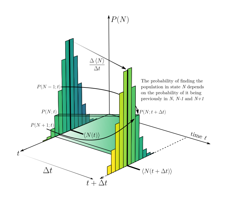
On this image we have 3 dimensions. The vertical one represents the probability $P(N)$ that the population is on the state $N$. Lower bars indicate lower probability. The other two axes on “the ground” indicate the time dimension and the specific state $N$. At the instant $t$, we notice that there are several values for $N$, with probabilities $P(N)$ greater than 0. When chosing one of these values of $N$, we compute the value for the probability of this value at time $t + \Delta t$ according to the equation above. On the image, there are two arrows indicating that $P(N+1;t)$ and $P(N-1;t)$ also afect the result of $P(N;t + \Delta t)$, as highlighted by the equation. We can then think that $P(N;t+\Delta t)$ depends on the probabilities that the population is at $N+1$, $N-1$ and $N$ at time $t$. Each probability is weighted by the chance that reproductions and deaths occur (or not). If we want to compute how this whole distribution changes from one moment to another, we need to compute $P(N;t+\Delta t)$ for all values of $N$.
Then, instead of asking ourselves about the chance that the population IS in a given value, it makes more sence to ask how this probability changes over time.
Frequently in nature, it is easier to explain why things change then to explain why they are in the exact way they are now.
To achieve that, we divide the probability by $\Delta$ and move the term $P(N;t)$ to the left-hand side of the equation, obtaining the rate of change for the probability over time
\[\begin{align} \frac{P(N;t+\Delta t) - P(N;t)}{\Delta t} &= -P(N;t)(b+d+\alpha)n + P(N-1;t)b(N-1) \\ \nonumber & + P(N+1;t)(N+1)(d + \alpha) + \mathcal{O}(\Delta t), \end{align}\]and as mentioned before, we are going to take the limit $\Delta t \rightarrow 0$, so that our rate of change represents “instantaneous” rates of change.
\[\begin{align} \lim_{\Delta t \rightarrow 0} \frac{P(N;t+\Delta t) - P(N;t)}{\Delta t} = \frac{\mathrm{d}}{\mathrm{d}t}P(N;t), \end{align}\]finally, we obtain
\[\begin{align} \boxed{ \frac{\mathrm{d}}{\mathrm{d}t}P(N;t) = -P(N;t)(b+d+\alpha)n + P(N-1;t)b(N-1) + P(N+1;t)(N+1)(d + \alpha) } \end{align}\]Aaahh look at this, a differential equation! Happly they are much more solvable and as Steven Strogatz once said:
“Since Newton, humanity has learned that the laws of nature are often expressed in the language of differential equations”
In fact this is exactly the master equation of this system!
However, this equation is still to complicated. Not to say that it is useless, it contains all the information necessary to describe the system, allowing us to conduct simulations and some mathematical analysis. But to our aim here, we need to simplify it more, because right now the probability of going to state $N$ depends on the probability of $N$ itself, $N+1$ and $N-1$. The probabilities for $N+1$ and $N-1$ will then depend on the probabilities of $N+2$, $N$, $N-1$ and $N-2$, $N$, $N-1$, respectively; and so on. In the end we will end up with a system of god knows how many coupled differential equations. For small values of $N$ this could be solvable, if we estabilish a maximum limit for the probability distribution of $N$, but it quickly becomes impractical for large values of $N$.
What if then, instead of asking about the probability of a specific value, we ask ourselves about the average behavior ![]() ? What if instead of looking at the probabilities of $N$ at a given moment $t$, we just ask what is the mean value of $N$ at that instant? Here comes our 5th assumption. The one that the system is homogeneous enough, such that the mean is representative of the whole population. This computation of the mean value of $N$ is represented on the image showed above by the strong lines that show the values of $\left \langle N \right \rangle$ at $t$ and $t + \Delta t$. That is, what we are assuming here is that the change in time of that mean is equivalent to the change in time of the whole distribution. For a discrete distribution, such as the values of a population, the average is given by
? What if instead of looking at the probabilities of $N$ at a given moment $t$, we just ask what is the mean value of $N$ at that instant? Here comes our 5th assumption. The one that the system is homogeneous enough, such that the mean is representative of the whole population. This computation of the mean value of $N$ is represented on the image showed above by the strong lines that show the values of $\left \langle N \right \rangle$ at $t$ and $t + \Delta t$. That is, what we are assuming here is that the change in time of that mean is equivalent to the change in time of the whole distribution. For a discrete distribution, such as the values of a population, the average is given by
Here the notation $\left \langle N \right \rangle$ means the average value of $N$ (or in statistical terms the expected value of $N$). Readers from physics are probably used to this notation and once again I ask sorry for my friends in biology for the mess in your head with all notations, but due to my training I find this writting more fluid and easy. It is worth noting that by writting $\left \langle N \right \rangle$ we actually mean $\left \langle N (t) \right \rangle$, but we are omitting the temporal dependence of $N$ to make the notation more clean. Some friends from statistics might be more used to representing this as $\bar{N}$.
We will now transform the master equation into a differential equation for the mean value of $N$. By multiplying the master equation by $N$ and summing over all possible states, we get
\[\begin{align} \frac{\mathrm{d}}{\mathrm{d}t} \left \langle N \right \rangle & = - (b + d+ \alpha) \sum_{N} N^2 P(N;t) + \\ \nonumber & + b \sum_{N} N^2 P(N-1;t) - \\ \nonumber & - b \sum_{N} N P(N-1;t) + \\ \nonumber & + (d + \alpha) \sum_{N} N^2 P(N+1;t) + \\ \nonumber & + (d+\alpha) \sum_{N} N P(N+1;t) \end{align}\]But now it seems the situation only got worse. Before we had a system of coupled differential equations and now we have a differential equation with a lot of sums??? Yes, but trust the process. If we manage to turn all of these sums into something of the sort $\displaystyle \sum_{N} N P(N;t)$, we will be able to rewrite everything in terms of the average $N$, since this is exactly the definition of mean. The first term of the equation is already in this format and we shall then pay attention to the second. If we rename the indexes of the sum from $N$ to a new index $M$, such that $M = N-1$ we rewrite the sum as
\[\begin{align} b \sum_{N} N^2 P(N-1;t) = b \sum_{M} (M+1)^2 P(M;t) \end{align}\]However, $M$ is just an index of sum, it doesn’t matter how we call it. We will then rename it back to $N$, in such a way that now
\[\begin{align} b \sum_{N} N^2 P(N-1;t) = b \sum_{N} (N+1)^2 P(N;t) \end{align}\]This may seem to be a nonsensical magic trick for some, so allow me to pause our derivation in order to explain what is happening here (those who don’t want to see it may keep reading after the —).
What we did here in practice was to move the sum 1 index behind. This may sound ilegal and freestyle, but let’s get a pratical example:
Assume $P(0) = 0.05$, $P(1) = 0.15$, $P(2) = 0.3$, $P(3) = 0.3$, $P(4) = 0.15$, $P(5) = 0.05$ and $P(N>5) = 0$. In this case
\[\begin{align} \nonumber & \sum_{N} N^2 P(N-1) = \\ & = \sum_{N=0}^\infty N^2 P(N-1) = 0\times P(-1) + 1^2 \times P(0) + \cdots + 6^2 \times P(5) + \cdots \end{align}\]naturally all terms from $P(6)$ forward will be null, just like the first term, since it deals with $P(-1)$, which is not defined here (our sum begins at 0), making it 0. The result of this sum is $13.7$. Nice, now let us do the change in index such that $M = N-1$. We now have
\[\begin{align} \nonumber & \sum_{N=0}^\infty N^2 P(N-1) = \\ & \sum_{M=-1}^\infty (M+1)^2 P(M) = 0^2\times P(-1) + 1^2 \times P(0) + \cdots + 6^2 \times P(5) + \cdots \end{align}\]Note that this is still the same sum. The result is still $13.7$. That happens because the relationship between the terms of the sum is still the same, as you may verify by writting term by term of the sum.
Expanding the recently found term of the sum, we write
\[\begin{align} b \sum_{N} (N+1)^2 P(N;t) & = b \sum_{N} N^2 P(N;t) + 2 b \sum_{N} N P(N;t) + b \underbrace{\sum_{N} P(N;t)}_{=1} = \\ \nonumber & = b \sum_{N} N^2 P(N;t) + 2 b \sum_{N} N P(N;t) + b, \end{align}\]where the in the last line we used the normalization condition $\sum_{N} P(N;t) = 1$. The sum at the third term becomes
\[\begin{align} b \sum_{N} N P(N-1;t) & = b \sum_{N} (N+1) P(N;t) = b \sum_{N} N P(N;t) + b \end{align}\]In analogy for the sums with $P(N+1;t)$, we make the change of index $M = N+1$ and obtain, after renaming it back to $N$
\[\begin{align} (d + \alpha) \sum_{N} N^2 P(N+1;t) & = (d + \alpha) \sum_{N} (N-1)^2 P(N;t) = (d + \alpha) \sum_{N} N^2 P(N;t) - \\ \nonumber & - 2 (d + \alpha) \sum_{N} N P(N;t) + (d + \alpha) \end{align}\] \[\begin{align} \nonumber (d + \alpha) \sum_{N} N P(N+1;t) & = \\ (d + \alpha) \sum_{N} (N-1) P(N;t) & = (d + \alpha) \sum_{N} N P(N;t) - (d + \alpha) \end{align}\]Bringing it all together, the master equation is written as
\[\begin{align} \frac{\mathrm{d}}{\mathrm{d}t} \left \langle N \right \rangle & = - (b + d+ \alpha) \sum_{N} N^2 P(N;t) + b \sum_{N} N^2 P(N;t) + 2 b \sum_{N} N P(N;t) + \\ \nonumber & + b - b \sum_{N} N P(N;t) - b + (d + \alpha) \sum_{N} N^2 P(N;t) - \\ \nonumber & - 2 (d + \alpha) \sum_{N} N P(N;t) + (d + \alpha) + (d + \alpha) \sum_{N} N P(N;t) - (d + \alpha) \end{align}\] \[\begin{align} \boxed{\frac{\mathrm{d}}{\mathrm{d}t} \left \langle N \right \rangle = b \sum_{N} N P(N;t) - d \sum_{N} N P(N;t) - \alpha \sum_{N} N P(N;t)} \end{align}\]Notice that if $b$, $d$ and $\alpha$ are constants, we may write
\[\begin{align} \nonumber &\frac{\mathrm{d}}{\mathrm{d}t} \left \langle N \right \rangle = (b - d- \alpha) \sum_{N} N P(N;t)\\ & \frac{\mathrm{d}}{\mathrm{d}t} \left \langle N \right \rangle = \underbrace{(b - d- \alpha)}_{r} \left \langle N \right \rangle, \end{align}\]and this equation becomes the same as a equation for exponential growth, with a difference that the total mortality term is now added a new factor due to intraspecific competition. Now instead of $b > d$ being the necessary condition for exponential growth, we need $b > d + \alpha$. If the reproduction rate of the population is higher than the sum of death rate by natural causes and death rate by intraspecific competition, then the population grows exponentially.
But the death rate by intraspecific competition is proportional to the probability that two individuals find the same source of food in order for them to fight over it. This means that if we consider $\alpha$ a constant, we are saying that this probability is always the same, regardless of the population size. This is only possible if space and resources are infinite. Then, the birth of a new individual does not prevent anyone else from reaching a food source. However, in reality this is not true. Naturally, the chance of encounter is proportional to the number of individuals. Thus a more realistic description would be to set the death rate by intraspecific competiton as a function of population size. The less individuals, the smaller the need to compete for food, water, space, etc. The specific form of this function will depend on a lot of things, for example the foraging behavior of individuals and spatial geometry, which will dictate what is exactly the probability of encounter for a given population size. However, in the spirit of starting with simple and general descriptions, we approximate the dependency of competition with population by a linear relationship $\alpha = \alpha_0 N$. That is, resource competition rises linearly with population size.
With this improvement only, keeping all other parameters as constants, we get
\[\begin{align} \frac{\mathrm{d}}{\mathrm{d}t} \left \langle N \right \rangle & = b \sum_{N} N P(N;t) - d \sum_{N} N P(N;t) - \alpha_0 \sum_{N} N^2 P(N;t) = \\ \nonumber & = b \left \langle N \right \rangle - d \left \langle N \right \rangle - \alpha_0 \left \langle N^2 \right \rangle . \end{align}\]which seems to be the differential equation for the logistic model, except that it requires the mean value of $N^2$, that is, the second statistical moment of the probability distribution of possible states of the system ![]() . We need to find $\left \langle N^2 \right \rangle$ in order to solve this equation. We could remake the whole process of multiplying by $N$ and adding the sum, but with $N^2$ in order to find the equation for $N^2$ and substitute. However, that equation would then depend on $\left \langle N^3 \right \rangle$, which wouldn’t help much.
. We need to find $\left \langle N^2 \right \rangle$ in order to solve this equation. We could remake the whole process of multiplying by $N$ and adding the sum, but with $N^2$ in order to find the equation for $N^2$ and substitute. However, that equation would then depend on $\left \langle N^3 \right \rangle$, which wouldn’t help much.
The mean field approximation also assumes that deep down, all statistical moments of the distribution of order bigger than 1 are given in terms of the first statistical moment (the mean). Thus
\[\begin{align} \boxed{\frac{\mathrm{d}}{\mathrm{d}t} \left \langle N \right \rangle = b \left \langle N \right \rangle - d \left \langle N \right \rangle - \alpha_0 \left \langle N \right \rangle^2 = \left \langle N \right \rangle \left[ \underbrace{(b-d)}_{r} - \alpha_0 \left \langle N \right \rangle \right]} \end{align}\]This is the known equation for the logistic model! ![]()
When analysing it, we may notice that
\[\begin{align} \nonumber & \frac{\mathrm{d}}{\mathrm{d}t} \left \langle N \right \rangle = 0 \Leftrightarrow \left \langle N \right \rangle = 0 \\ \nonumber & \text{or} \\ \nonumber & \frac{\mathrm{d}}{\mathrm{d}t} \left \langle N \right \rangle = 0 \Leftrightarrow \left \langle N \right \rangle = \frac{r}{\alpha_0} \end{align}\]That is, the population stops growing ($\mathrm{d} \left \langle N \right \rangle / \mathrm{d}t = 0$) either if the population is $0$ (everyone is dead) or when it reaches the value $r/\alpha_0$. Since $r/\alpha_0$ is bigger than 0, this ration sets a maximum for the size of the average population size. We call it carrying capacity $k$. By writting $\left \langle N \right \rangle = n$, just to make the notation clean and state that the population size $n$ here is the expected value of it, we arrive at the version of the logistic model we saw at the beginning of this text
\[\begin{align} \frac{\mathrm{d}n}{\mathrm{d}t} = rn \left(1 - \frac{n}{k} \right) \end{align}\]Deep down, the mean field approximation is telling us that the variance in the probability distribution of $N$ is negligible. $\mathrm{Var}[N] = \left \langle N^2 \right \rangle - \left \langle N \right \rangle^2 = 0 \Rightarrow \left \langle N^2 \right \rangle = \left \langle N \right \rangle^2$. If the variance was not negligible, than we could rewrite the equation as
\[\begin{align} \frac{\mathrm{d}}{\mathrm{d}t} \left \langle N \right \rangle = b \left \langle N \right \rangle - d \left \langle N \right \rangle - \alpha_0 \left( \left \langle N^2 \right \rangle + \mathrm{Var}[N] \right) \end{align}\]That means that the presence of a spread in the probability distribution of states for this system, naturally induces a change in the expected value of $N$ for a given time $t$. This means that stochasticity not only creates fluctuations around the mean, but it is also capable of changing the expected value itself.
We now arrive at the end of this derivation and found the famous equation for the logistic model. It is worth taking a breath to reflect on some things:
The first of them is that we had to assume 5 things to arrive on it:
- Individuals only interact with their food and amongst themselves
- Reproduction is assexual
- All individuals have the same fitness
- Death, reproduction and competition occur independently from each other
- The system is spatially homogeneous
And on top of this the extra assumption that the variance in the state probability of $N$ is negligible and that the competition rate is linearly proportional to the population size $\alpha = \alpha_0 N$.
Many things had to be assumed for us to get to this equation. In a lab, it is “easy” to achieve these requirements, which makes the verification of this equation more tangible. That however, does not turn the equation useless outside the lab, in real life, for it serves as a base to build descriptions on the behavior populations on it’s most basic level. Later we can divide the population into males $M$ and females $F$, and assume sexual reproduction, for example. Eliminating that assumption. Each one of them may be tackled individually to approximate the model from reality.
In fact, some of these assumptions are what may be called “weak” assumptions. Meaning that their requirement is not central to the qualitative behavior described by the equation. For example, sexual reproduction requires individuals with different sexes, but adding it to the model does not change the fact that populations start growing fast and eventually reach a plateau given a constant environmental condition and absence of other competitors. In fact, depending on the timescale we look at, and the composition of the population, even a sexual reproduction that it’s not instant may be treated as a assexual instant phenomena. For example, suppose that sexual reproduction takes some time $\delta$ to occur. If $\delta$ is negligible in the timescale studied and the population has a somewhat equal share of males and females, then population growth will be proportional to the current population size, which is not different than what we get by assuming assexual reproduction. That happens because the scale of the assumption is much smaller than the scale of the system, and it’s violation does not affect the system. This discussion is a reminder that in mathematics assumptions are not statements about reality, but instead they are statements about what is approximately equivalent to reality under the specifics of the system at hand.
But all of it then begs the question:
But what is the purpose of a model?
Is it’s only purpose to describe reality with the biggest precision possible? Or does it serve as a tool to understand the role of several mechanisms that act on a system? If your answer tends to the first otpion than I fear no model (be it mathematical or not) will ever satisfy you. Now if you believe in the second option we begin to see the use of the logistic model. When we observe a system that obeys the logistic model fairly well, does that mean that all 5 premisses are satisfied? No! But it does mean that other mechanisms present are not so dominant in the life of individuals making up this population.
As an example, I will bring the reader to my mother field, physics. When we learn physics at school we always neglect air resistence. Why? Why spending years learning physics formulas and laws that do not describe the current world that we encounter everyday? There are two reasons for that, I believe. The first is difficulty. It is much easier to start with the simpler case (and we already see how much trauma it causes to students). Adding air resistence to a parabolic throw of an object, means to solve a second order differential equation
\[\begin{align} \frac{\mathrm{d}\vec{v}}{\mathrm{d}t} = -\vec{g} - \frac{1}{2} \rho C_d A \vec{v}^2, \end{align}\]in which I find reasonable to argue that students in high school do not have the maturity to comprehend and interpret.
The second reason is related to mechanisms. Yes, of course air is always present, but it is not air that rules the majority of the trajectory of a boll thrown in the air most of the times. Who dictates that is gravity. Air resistence plays a role so small under these scenarios that teaching students to solve differential equations just to find the trajectory of a ball thrown in the air during an american football match becomes equivalent of killing a fly with a balistic missile. It becomes more of a distraction of what really shapes this movement, than a valuable addition to the students knowledge about the functioning of the world.
The logistic model plays the same role in ecology. It is the ecological equivalent of mechanics without air resistence, rotation, electric charge and all else. But it is through it that we learn some general behaviors.
As a final note, in the case of air resistence, the description without it is so good that many times, we don’t even need to account for it unless we are looking for an extra precision. Let’s say we want to measure the reach of a ball kicked by a football player during the world cup. If our measurement has an error of $\pm 10$ cm and inclusion of air resistence in the model predicting where the ball lands adds $4$ cm of accuracy, then this higher accuracy falls below the error of our measurement, making it undetectable. We just wasted effort.
In ecology that happens many times, some interactions between individuals are always present, but depending on the timescale and precision that we care, they become negligible.